Page 64 - MSc_thesis_R A Kil

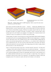
(a) Training image used in the MPS algorithm. (b) Intersected training image in order to illustrate
internal architecture.

Figure 6.1 – Training image grid for the MPS algorithm. North is upper left, facies colour
according to general facies legend.

those regions is thereafter modelled with a separate — stationary — training image. Modelling eastern
Favignana with the concept of regions would imply a clear boundary between the different regions that
is not observed in this fieldwork campaign. Moreover, the complex internal architecture that exists
throughout the island is not suitable for this type of modelling. Instead, an approach with a single
training image for the entire fieldwork area is suggested. The thoughts of the conceptual geological model
- described in section 5 are attempted to be included in this training image.

Training images can be given in various formats such as hand-drawn sketches, digital (areal) photographs,
or basically any 3D model one can imagine (Schlumberger, 2009). The ideal training image is a rectangular
3D grid, which will be used in this modelling exercise as well. The Petrel software package offers the
option to draw arbitrary facies patterns in a grid. Filters on i, j or k values are used to address facies
only to designated grid cells. The most convenient method was to filter every k layer, and draw the
desired facies positions for each layer separately. The training image grid can then be quality-checked
with intersections in a three dimensional view.

Figure 6.1 shows the final training image used to model the Favignana calcarenite. The entire block
— consisting of 100 by 125 by 20 grid cells with a size of one metre in all directions — as well as an
intersected grid is shown. It is attempted to include the interpreted depositional environment as described
in the conceptual geological model. Because the training image cannot include too much variation, one of
the conditions was that only two facies can be next to each other in a single k layer. Some examples of
intermediate k layers are given in figure D.2 in appendix D. The images show an attempt to include the
propagating nature of the calcarenite complex, with preferred orientation to the southeast.

46