Page 9 - ENERGIA_MARE

Author's personal copy
946 L. Liberti et al. / Renewable Energy 50 (2013) 938e949
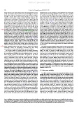
Island and near San Pietro Island; along the intermediate section
of the coast lower values between 8.5 and 10 kW/m are found.
Around the northern and southern limit of the western Sardinia
coastline average wave power drops sharply as soon as the
exposure to the waves coming from W and NW declines. The
north-western and southern coasts of Sicily have a lower potential
with average wave power ranging between 2.5 and 6.5 kW/m. On
the northern coast west of Palermo average wave power flux is
between 4 and 5 kW/m gradually increasing to values between 5
and 6 kW/m between San Vito Lo Capo and Trapani. The most
productive area is located along the coastal stretch that lies north
of Mazara del Vallo where average power is above 6 kW/m
reaching values around 7 kW/m near Favignana Island. The rest of
the southern coast is the least productive with average power flux
below 4.5 and as low as 2.5 kW/m. The only exception is the area
between Punta Secca and Capo Passero where values are almost
everywhere near 5 kW/m. Similarly to what was previously
observed on the Sardinia coast there is a sharp decline in average
power east of Palermo and north of Capo Passero. Figs. 9 and 10
show that average wave power exhibits a non-negligible spatial
variability even at spatial scales of the order of 20 km. For
instance, the average wave power just a few kilometers south of
Alghero decreases almost 20%. Similar spatial variations can be
observed around San Pietro Island in Sardinia and near Mazara del
Vallo, Favignana Island and Punta Secca in Sicily. Such spatial
variability cannot be adequately described by local buoy
measurements or by models with lower spatial resolution.
The average power is a useful parameter to identify promising
areas for wave energy production, however, its values arise from
the contribution of individual sea states distributed over a range of
wave heights, periods and directions. The power of the most
energetic and less frequent sea states can easily be more than one
order of magnitude greater than the values observed in typical
conditions. From an engineering point of view, since the WECs
effectively operate on specific ranges of wave heights and periods,
the feasibility study for wave energy production should be carried
out considering the most representative sea states in terms of
energy production. Wave power associated to the less frequent and
most energetic states cannot be taken into account since its
exploitation requires over-dimensioned infrastructures and the use
of WECs that probably are not able to perform well in less energetic
sea states. Directional distribution of wave energy should also be
considered for non-point absorber devices. In Figs. 11 and 12 is
provided an overview of the spatial variability of the distribution of
wave power among heights, periods and directions at selected
locations along western Sardinia, north-western and southern
Sicily. In the lower left panel of the figures, the scatter plot repre- a pattern where the winter and fall seasons are the most energetic
sents the distribution of yearly average energy in terms of Te and Hs, and calmer sea states are normally observed during the rest of the
evaluated over the 10 years simulated period. Contribution to the
total energy given by individual sea states are lumped together in
0.25 s intervals of Te and 0.25 m intervals of Hs. Wave power
contributions of individual 3-h sea states obtained from the model
output are calculated using Equation (11). Lines of constant power
are drawn on the scatter plots to highlight wave power variability.
On the upper and right panels of each scatter plot two histograms
represent the distribution of average yearly wave energy over Te
and Hs respectively. The intervals used in the histograms are twice
the size of the intervals used in the scatter plot for better graphic
Fig. 11. Distribution of wave energy as a function of significant wave period and significant wave height at points located along the western coast of Sardinia (see Fig. 9 points 1.ae
1.f). The lower left panel of each figure shows the average yearly energy associated with sea states identified by Te and Hs couples. Dotted lines mark reference power levels. Upper
panel shows the energy distribution as a function of Te only; right panel as a function of Hs only. Lines in the upper and right panels are the cumulative energy as a percentage of the
total. Dots on the cumulative lines mark each 10th percentile. Rose plot in the upper right panel shows energy distribution over wave incoming direction.
representation. In each histogram a line represents the cumulative
percentage of total energy available in terms of Te and Hs. Markers
are placed every 10th percentile on the cumulative line. In the
upper right panel a rose diagram describes the directional distri-
bution of average yearly energy over 30 wide direction bins. Each
concentric circle represents 20% contribution to the total wave
energy. The plots in Fig. 11 refer to points located along western
Sardinia coast (see Fig. 9). Sea states with significant wave heights
between 2 and 4 m and significant periods between 8 and 10 s
appear to carry a considerable amount of the total energy, both
around 40%. There are however some notable differences between
the various locations. Points 1.a and 1.b, located in the northern
section of the coastline, only 50 km away, have similar values of
average power flux and its distributions among Te and Hs are also
nearly the same, however the directional distribution appears to be
quite different with dominant directions shifted almost 45 apart.
In these two locations the amount of power provided by the most
extreme sea states, with Hs above 4 m, is around 40% of the total,
while in the remaining locations this contribution reduces to about
30%. This is observed for points 1.c and 1.d, which are far less
energetic than point 1.a and 1.b, but also for points 1.e and 1.f which
share the same power levels of the first two points. Similarly, points
1.c and 1.d have the same energy content but different directional
distributions.
The wave energy distribution along points located off the Sicily
coast follows a different pattern as shown in Fig. 12. Here the most
energetic contributions in terms of significant period, accounting to
50% of the total, are located at lower values of Te, in the range
between 6 and 8 s. Likewise, the main contribution to total energy
in terms of Hs, reaching 50% of the total, is found in a lower range of
values between 1.5 and 3.5 m. The main differences among the
plots shown in Fig. 12 are in the wave energy directional distribu-
tion which has a prevalent NWW component but appears more or
less scattered depending on the location. Points 2.e and 2.f have
similar energy contents but directional distribution is extremely
different with a concentrated distribution at point 2.e and a more
scattered one at point 2.f. Furthermore, wave energy at these two
locations is distributed in a narrower Hs band, when compared to
the other points, with almost 70% of the total energy in the range
between 1 and 3.5 m.
3.3. Wave power variability
As a final remark we observe that temporal distribution of wave
energy also plays an important role in the site selection. In the
Mediterranean the seasonal distribution of sea states follows
year [23]. The seasonal variability of the wave power flux we
calculated shows a similar trend. Fig. 13 shows the spatial distri-
bution of seasonal average power flux in the Mediterranean for the
entire simulation period. As expected, the winter months of
December, January and February are the most productive followed
by the autumn ones. Wave power spatial distribution follows
approximately the pattern described for the yearly average. Some
differences can be found in the Central Mediterranean which
appears to be especially energetic during the winter season and
calm during the summer. The seasonal average power exhibits