Page 6 - Lovison_alii_2010

MODELING POSIDONIA OCEANICA GROWTH DATA

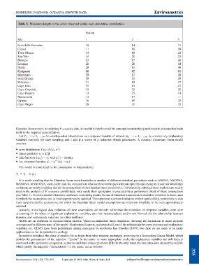
Table 3. Maximum length of the series observed within each site/station combination

Station
Site 1 2 3
Isola delle Femmine 10 14 31
Capaci 11 16 18
Torre Muzza 14 18 23
San Vito 14 21 21
Bonagia 23 17 20
Levanzo 28 20 14
Nubia 20 11 48
Favignana 22 27 21
Marettimo 29 17 18
Isola Grande 30 21 29
Petrosino 21 18 17
Capo Feto 35 15 21
Capo Granitola 19 22 20
Capo Passero 13 25 13
Marzamemi 12 17 —
Ognina 16 19 22
Capo Negro 20 21 23

Gaussian linear models in analyzing P. oceanica data, it is useful to briefly recall the assumptions underlying such models, in a way that lends
itself to the required generalization.
Let Y i ; i ¼ 1; .. .; n; be n independent observations on a response variable of interest, x i ; i ¼ 1; ...; n; be a vector of p explanatory
variables available for each sampling unit i and b a vector of p unknown (fixed) parameters. A classical (Gaussian) linear model
assumes:
2
error distribution Y i jx i Nðm i ; s Þ
T
linear predictor h i ¼ x b
i
link function gðm i Þ¼ h with gðÞ ¼ identity
i
1
(or, response function m i ¼ g ðh i Þ¼ h i Þ
The model is completed by the assumption of independence:
ƒ 8i 6¼ j
Y i Y j
It is worth recalling that the Gaussian linear model underlies a number of different statistical procedures such as ANOVA, ANCOVA,
MANOVA, MANCOVA, t-test, and F-test. So, even authors who use these techniques without explicitly specifying the model on which they
are based, are tacitly implying that all the assumptions of the Gaussian linear model hold. Unfortunately, although these methods are widely
used in the analysis of P. oceanica growth data, only rarely their application is preceded by a preliminary check of these assumptions
(see Table 1). To avoid invalid inferences, and hence misleading results, the use of Gaussian linear models should be restricted to those cases
for which the assumptions are, at least approximately, satisfied. This represents a serious limitation to their applicability, particularly to data
from natural complex ecosystems, for which the Gaussian linear model assumptions are often too simplistic to be even approximately
satisfied.
Actually, in ecological data violations of these assumptions are the rule rather than the exception: (i) response variables, even after
accounting for the effect of significant explanatory variables, are often heteroscedastic and/or non-Normal; (ii) the relationship between
response and explanatory variables are often nonlinear.
GLMs are an extension of classical linear models, which accommodate these departures, allowing the statistician to make separate
assumptions for different parts of the model: distributional aspects, mathematical form of the relationship between response and explanatory
variables, etc. GLM’s have been popularized among ecologists by textbooks like Crawley (1993), but there do not seem to be many
applications so far in quantitative ecology.
In order to introduce this class of models, let us begin from what remains unchanged in moving to a Generalized Linear Model, which
justifies the permanence of the adjective ‘‘Linear’’ in the name: at some appropriate scale, the explanatory variables are still linearly
T
combined in the systematic component, so that we still have a linear predictor x b. On the other hand, the two extensions allowed by a GLM,
i
which justify the adjective ‘‘Generalized’’ in the name, are as follows: 375

Environmetrics 2011; 22: 370–382 Copyright ß 2010 John Wiley & Sons, Ltd. wileyonlinelibrary.com/journal/environmetrics