Page 9 - Rouyer_Fromentin_2008

Rouyer et al.: Wavelet analysis of multiple time series 19

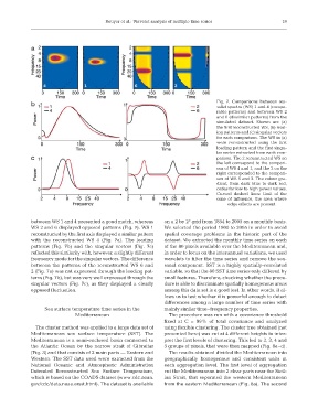
Fig. 7. Comparisons between wa-
velet spectra (WS) 1 and 4 (compa-
rable patterns) and between WS 2
and 6 (dissimilar patterns) from the
simulated dataset. Shown are (a)
the first reconstructed WS, (b) lead-
ing patterns and (c) singular vectors
for each comparison. The WS in (a)
were reconstructed using the first
leading pattern and the first singu-
lar vector extracted from each com-
parison. The 2 reconstructed WS on
the left correspond to the compari-
son of WS 4 and 1, and the 2 on the
right corresponded to the compari-
son of WS 6 and 2. The colour gra-
dient, from dark blue to dark red,
codes for low to high power values.
Curved dashed lines: limit of the
cone of influence, the area where
edge effects are present

between WS 1 and 4 presented a good match, whereas on a 2 by 2° grid from 1854 to 2005 on a monthly basis.
WS 2 and 6 displayed opposed patterns (Fig. 7). WS 1 We selected the period 1900 to 2005 in order to avoid
reconstructed by the first axis displayed a similar pattern spatial coverage problems in the historic part of the
with the reconstructed WS 4 (Fig. 7a). The leading dataset. We extracted the monthly time series on each
patterns (Fig. 7b) and the singular vectors (Fig. 7c) of the 80 pixels available over the Mediterranean and,
reflected this similarity with, however, a slightly different in order to focus on the interannual variations, we used
frequency mode for the singular vectors. The difference wavelets to filter the time series and remove the sea-
between the patterns of the reconstructed WS 6 and sonal component. SST is a highly spatially-correlated
2 (Fig. 7a) was not expressed through the leading pat- variable, so that the 80 SST time series only differed by
terns (Fig. 7b), but was very well expressed through the small features. Therefore, checking whether the proce-
singular vectors (Fig. 7c), as they displayed a clearly dure is able to discriminate spatially homogenous areas
opposed fluctuation. among this data set is a good test. In other words, it al-
lows us to test whether it is powerful enough to detect
differences among a large number of time series with
Sea surface temperature time series in the mainly similar time–frequency properties.
Mediterranean The procedure was run with a covariance threshold
fixed at C = 99% of total covariance and analyzed
The cluster method was applied to a large data set of using flexible clustering. The cluster tree obtained (not
Mediterranean sea surface temperature (SST). The presented here) was cut at 4 different heights to inter-
Mediterranean is a semi-enclosed basin connected to pret the first levels of clustering. This led to 2, 3, 4 and
the Atlantic Ocean by the narrow strait of Gibraltar 5 groups of pixels, that were then mapped (Fig. 8a–d).
(Fig. 3) and that consists of 2 main parts — Eastern and The results obtained divided the Mediterranean into
Western. The SST data used were extracted from the geographically homogenous and consistent units at
National Oceanic and Atmospheric Administration each aggregation level. The first level of aggregation
Extended Reconstructed Sea Surface Temperature, cut the Mediterranean into 2 clear parts near the Sicil-
which is based on the COADS dataset (www.cdc.noaa. ian Strait, that separated the western Mediterranean
gov/cdc/data.noaa.ersst.html). The dataset is available from the eastern Mediterranean (Fig. 8a). The second