Page 5 - Rouyer_Fromentin_2008

Rouyer et al.: Wavelet analysis of multiple time series 15

n−1
decomposition is more general than the eigenvalue DL ,L = ) ∑ atan[ ( L t ()− L t ())−( k ( k ( 1))]
(
k
k
k
k
j
i
decomposition used for principal component analysis, i j i j L t +11)− Lt +
t=1
but the 2 decompositions are nevertheless related. A (8)
k
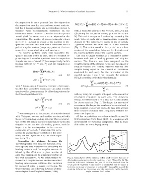
singular value decomposition performed on the with n being the length of the vectors, and L i (t) and
k
covariance matrix between 2 similar wavelet spectra L j (t) being the kth pair of leading patterns for W i and
would yield the same results as an eigenvalue de- W j . This metric compares 2 vectors by measuring the
composition. The number of non-zero singular values angle between each pair of corresponding segments,
(k) of ΓΓ is inferior or equal to the number of fre- defined by the consecutive points of the 2 vectors;
quencies analysed and each one is associated with a 2 parallel vectors will thus lead to a null distance
pair of singular vectors (frequency patterns), that are (Fig. 2). This metric could be interpreted as a robust
respectively associated with each spectrum. version of the correlation between the derivatives of
The leading patterns show how respective fre- the leading patterns and/or the leading vectors.
quency patterns evolve in time, and are obtained by The sum of angles obtained is a comparable metric
projecting each wavelet spectrum onto its respective between each pair of leading patterns and singular
k
k
singular vectors. L i (t) and L j (t) are respectively the kth vectors. The distance was then computed as the
leading patterns for W i and W j , and are computed as weighted mean of the distance for each of the k pairs of
follows: singular vectors and leading patterns retained (the
ƒ =F weights being equal to the amount of covariance
()
k
Lt = ∑ U k × W (ƒ ,t ) explained by each axis). For the comparison of the
i
i
ƒ =1
and (6) wavelet spectra i and j, we compute the distance
ƒ =F DT(i,j) according to the following formula:
()
k
Lt = ∑ V k × W (ƒ ,t ) k=K
j
j
)
(
ƒ =1 ∑ w ×( D L ,L + D(UV j k ))
k
k
k
,
k
i
i
j
(
)
with F the maximum frequency common to both spec- DT i, j = k=1 (9)
k=K
tra. It is then possible to reconstruct the initial wavelet ∑ w k
spectra with a given number, N, of leading patterns by k k=1
the following relationships: with w k being the weights, set equal to the amount of
covariance explained by each axis. The distances,
k=N
k
W i N = ∑ U × L k i DT(i,j), were then used to fill a distance matrix suitable
k=1 for cluster analysis (Fig. 1). The larger the amount of
and (7)
k=N covariance, the larger the number of axes retained; a
k
W j N = ∑ V × L k j large number of axes will enable to take into account
k=1 more detailed common time–frequency features be-
These correspond to the product of a matrix formed tween the 2 spectra.
with N singular vectors and another one formed with All the computations were done using R version 2.4
the N corresponding leading patterns. The reconstruc- (R Development Core Team [2006] R: a language and
tion for the kth axis is therefore determined by the kth environment for statistical computing). This is avail-
singular vector and the kth leading pattern, and the able online at: www.R-project.org.
larger k is, the less important is the common
covariance explained. A reconstruction corre-
sponds to a filtered representation of the spec-
trum; the less important N is, the more impor-
tant is the filter.
Computing the distance between the
wavelet spectra: The distance between 2 wa-
velet spectra was measured by comparing the
leading patterns and the singular vectors ob-
tained by the MCA over a given number of
axes (that correspond to a fixed percentage of
the total covariance). As the relationships be- Fig. 2. Computation of the distance index used between the pair of
k
k
tween the 2 singular vectors and between the 2 kth leading patterns (or singular vectors), L i and L j (see Eq. 8). The
absolute difference between the pair of vertical dashed lines for
leading patterns were not linear, they could not
every pair of segments of the 2 series is computed and the angle a,
be compared using a simple correlation. We
between each pair of segments is obtained by taking the atan of the
thus computed the following distance (D) mea- absolute differences. Summing over the segments yields the total
sure adapted from Keogh & Pazzani (1998): angle between the 2 series