Page 7 - Rouyer_Fromentin_2008

Rouyer et al.: Wavelet analysis of multiple time series 17

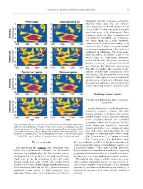
dominated by low-frequency oscillations,
whereas white noise does not produce
such highly autocorrelated signals. On the
contrary, the Fourier surrogates identified
significant areas in the whole range of fre-
quencies. However, their locations were
sometimes not consistent (e.g. Portoscuso),
and many small areas were identified.
These spurious effects were likely to be
created by the Fourier surrogates applied
on short and non-stationary time series, as
explained in ‘Methods’. The beta surro-
gates identified significant areas in the
whole range of frequencies. However,
unlike the Fourier surrogates, the size of
the time series and its non-stationarity did
not influence the algorithm used to pro-
duce the surrogates. The locations of sig-
nificant pseudo-cyclic components were
well defined, and no spurious effects were
detected. This approach thus allowed us to
identify cycles significantly different from
the expected behaviour of ecological time
series displaying similarly coloured noise.

Clustering wavelet spectra
Signals with determined time–frequency
properties

In order to illustrate how the classification
procedure extracts common time–fre-
quency patterns to compare the wavelet
spectra, we first formed a data set with time
series displaying known and controlled
properties in time and frequency. Six time
Fig. 4. Wavelet spectra of the Formica and Portoscuso time series, tested with series displaying contrasting time–fre-
different null hypotheses. We used a white noise process, an AR[1] process, the
Fourier surrogates (Type I) and our class of surrogates (Beta surrogates). Solid quency properties were simulated, using
black lines indicate significant areas at the 5% level. The colour gradient, from sine and cosine functions (Fig. 5). The
dark blue to dark red, codes for low to high power values. Curved dashed lines: changes in frequency were either abrupt
limit of the cone of influence, the area where edge effects are present (Fig. 5, time series 2, 3, 5 and 6) or smooth
(Fig. 5, time series 1 and 4). Indeed, these
Time series results time series displayed different dynamics compared to
real ecological time series or outputs from models (e.g.
The results for the Formica and Portoscuso time a stochastic version of the Ricker model). However,
series are presented to illustrate the differences they allowed us to control both the time and frequency
between the methods (Fig. 4). The wavelet spectra properties of the time series, and we could thus obtain
displayed different significant areas (indicated by solid wavelet spectra with desired time–frequency patterns.
black lines in Fig. 4), according to the null model The dataset with determined time–frequency prop-
against which they were tested. The spectra tested erties was first analysed using wavelet analysis (Fig. 6).
against white noise displayed large significant areas at The wavelet spectra (WS) displayed clearly different
low frequencies, whereas the AR[1] process identified patterns: (1) an increase in frequency with time; (2) a
significant areas mostly at high frequency (e.g. decrease in frequency with time; and (3) continuous
Formica). These results were expected; an AR[1] is patterns.