Page 4 - Rouyer_Fromentin_2008

14 Mar Ecol Prog Ser 359: 11–23, 2008

β
the 1/ƒ model, and the phases are drawn by a uniform onal elements are the singular values; they are dis-
variable on the interval (0, 2π). A back transformation posed in decreasing order of magnitude, and they
with the inverse Fourier Transform (Voss 1988) are proportional to the squared covariance accounted
produces the surrogates. Using this approach, we thus for each axis. Each singular value is thus associated
obtain surrogates that mimic the shape of the original to common patterns of decreasing importance
ecological time series by displaying a power spectrum between the 2 spectra. The singular value decompo-
with the same slope, but without exactly reproducing sition finds an orthonormal basis for each spectrum,
it. determined by their respective singular vectors maxi-
Comparing the wavelet spectra with the MCA mizing their mutual covariance. The singular value
method. The maximum covariance analysis: Many
ecological time series, especially from the marine
environment, such as phytoplankton, zooplankton or
fisheries time series, contain a substantial amount of
zeros together with periods of low variability. This
leads to wavelet spectra that often display areas with
poor, or even without, power. As a consequence, a
direct comparison of the wavelet spectra will lead to a
classification that could be driven by the areas with
poor power. We addressed this by focusing on the com-
mon time–frequency properties between the pairs of
wavelet spectra, extracted by the MCA. The MCA,
historically called ‘singular value decomposition’
(Bretherton et al. 1992), has been widely used in mete-
orology to compare spatio-temporal fields (von Storch
& Zwiers 1999). The MCA is close to a combined
empirical orthogonal function analysis, but with a bet-
ter efficiency and robustness. It relies on a singular
value decomposition (which here designs the solution
of the matrix problem) performed on the covariance
matrix between 2 spatio-temporal fields. The first axis
of the MCA thus corresponds to the largest fraction of
the covariance between the 2 fields, which in this case
will be the wavelet spectra (for more details on MCA,
see Newman & Sardeshmukh 1995, Cheng & Dunker-
ton 1995). In other words, the first axis extracts the
most important common pattern between the 2 fields.
Constructing the covariance matrix implies, as an
underlying assumption, that the frequencies composi-
tions at different times are independent. This is gener-
ally not true but, like the eigenvalue decomposition,
the singular value decomposition is rather robust to
such bias and is therefore often used in this context
(e.g. Cheng & Dunkerton 1995). We compute the
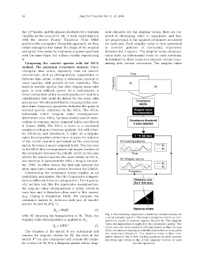
covariance matrix R i,j between each pair of wavelet
spectra W i and W j (Fig. 1):
R= W W t (4)
i,j i j
t
with W j denoting the transposition of W j . Then, the Fig. 1. Methodology employed to build the distance matrix for
a set of wavelet spectra. The cross-covariance matrix is com-
singular value decomposition is applied on R i,j : puted for a pair of wavelet spectra W i and W j . The singular
value decomposition is applied to the covariance matrix. The
R i,j = U ΓΓV t (5)
k first axes are then extracted, k being chosen so that the sum
The columns of the matrix U are orthogonal and of the covariance associated with the axes is below or equal to
the covariance threshold. The distance index is then com-
contain the singular vectors for W i ; the rows of the puted between the k first leading patterns of each wavelet
t
matrix V are also orthogonal and contain the singu- spectrum and between the k first singular vectors of each
lar vectors for W j . ΓΓ is a diagonal matrix whose diag- wavelet spectrum