Page 9 - EAI-4_2015_48-59

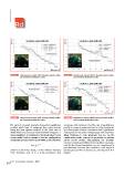
FIGURE 10 *HSH(aa\YYH[YHUZLJ[*( :\Y]L`LKILHJOWYVÄSLZ FIGURE 12 3PKV)\YYVUL[YHUZLJ[3):\Y]L`LKILHJOWYVÄSLZ
HUK[OLVYL[PJHSLX\PSPIYP\TWYVÄSL HUK[OLVYL[PJHSLX\PSPIYP\TWYVÄSL

FIGURE 11 *HSH(aa\YYH[YHUZLJ[*(:\Y]L`LKILHJOWYVÄSLZ FIGURE 13 3PKV)\YYVUL[YHUZLJ[3):\Y]L`LKILHJOWYVÄSLZ
HUK[OLVYL[PJHSLX\PSPIYP\TWYVÄSL HUK[OLVYL[PJHSLX\PSPIYP\TWYVÄSL

For each of surveyed transects, theoretical equilibrium increases with sediment size. The use of equilibrium
profiles which best fit measured data were derived profile to compare measured data is to be considered
using the least squares method. In the ideal case in as a first approximation, consistent with a qualitative
which there is no net cross-shore sediment transport, i.e. description of the coastal morphology and dynamics.
same magnitude of constructive and destructive forces, Main criticisms to this approach can be: (a) the
beach profile tends to assume a concave configuration, equilibrium profile concept is applicable to uniform
classically described by Dean [30] with a power function: sandy beach profile, disregarding the possible
presence of rock and differences in seafloor coverage,
where h is the water depth, x is the offshore distance and (b) the Dean formulation can be considered to
from shoreline and A is a scale parameter that progressively become less realistic as the depth of
submerged profile increases (i.e., starting from 6 m
depth).

54 EAI Energia, Ambiente e Innovazione 4/2015