Page 6 - LoRe_Musumeci_alii_2014

C. Lo Re et al. / Procedia Engineering 70 ( 2014 ) 1046 – 1054 1051

where P s is the exceedance probability of wave run-up (e.g for R 2% P s = 0.02).
5. Results

In the present work, we present a comparison of the numerical model results with the field measurements of a
video monitoring station installed on a tripod near the reference transect (Fig. 4), which acquired coastal zone
th
imagery from 11:30 to 15:30 of 29 march 2011. For this study the measured data was grouped every 30 minutes
in order to calculate the statistical run-up parameters. The simulated irregular wave train (30 min) was extracted
from a TMA spectrum with significant wave height and peak period equal to those obtained from the SWAN
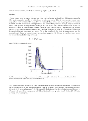
model. Fig. 5 shows an example of the spectrum of random waves extracted from a TMA spectrum with H s=0.86
and T p=6.16. The spatial domain of the Boussinesq model was discretized by using Δx = 1 m and t =Δ T 300s and
the numerical internal wavemaker was located 300 m far from beach. For both the measurements and the
numerical results the run-up parameters were calculated using equation (6). Whereas the significant wave run-up
was calculated using the following expression:

R = 4⋅ V ( )R + R (7)
s 100
where V(R) is the variance of run-up.

Fig. 5. The wave spectrum of the input random waves and the TMA spectrum (H s=0.86, T p=6.16 ). The continuous bold line is the TMA
spectrum the light line is the random wave spectrum without smoothing.

Fig. 6 shows the result of the numerical model for a train of random wave, obtained by assuming a TMA spectrum
and H s=0.86 and T p=6.16. The shoreline horizontal position values for this simulation were varying between -
4.64 m<ξ<11.30 m around a mean of 1.94 (Fig. 6a), while the horizontal shoreline velocity fluctuated from u s = -
3.79m/s to 3.23 m/s with the average equal to 0.002m/s(Fig. 6b). The run-up varied from R=-0.32 and R=0.79 with
an average of 0.14 m (Fig. 6c).