Page 4 - Power_Line_Cataliotti_2012

CATALIOTTI et al.: PLC IN MV SYSTEM 65

Fig. 7. Elementary cell of a transmission line.

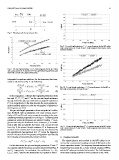
Fig. 9. Per-unit-length inductance versus frequency for the MV cables

with a cross section of 25 and 50 mm . Both frequency trends can be easily
assumed constants.

Fig. 8. Per-unit-length resistance versus frequency for the MV cables

with a cross section of 25 and 50 mm . The experimental measurements were
fitted with a second-order polynomial function.

telegrapher’s equations which are, for the elementary line trans-
mission cell shown in Fig. 7, the following:

(1) Fig. 10. Per-unit-length conductance versus frequency for the MV ca-

bles with a cross section of 25 and 50 mm .
(2)

In these equations, denotes the longitudinal direction of the
line and , , , and are the per-unit length resistance
( ), inductance ( ), conductance ( ) and capacitance
( ), respectively. In the time domain, the most popular nu-
merical method applied to solve the telegrapher’s equations is
the Bergeron one [11].
The per-unit length parameters of two unipolar MV cables,
type RG7H1R with an aluminum core cross section, respec-
tively, of 25 and 50 mm , were measured according to the mea-
surement procedure proposed in [7]. In Figs. 8–11, the measured
parameters versus the frequency are plotted. Usually, is ne-
glected and only the distributed series resistance is consid-
ered to take into account the line losses [11]. As can be seen
Fig. 11. Per-unit-length capacitance versus frequency for the MV cables
from Fig. 8, the per-unit length resistance is frequency de-
with a cross section of 25 and 50 mm . Both frequency trends can be easily
pendent and a variation law versus frequency was obtained by assumed constants.
the experimental measurements [11]. versus the frequency
trend in the case of the line-ground configuration was fitted by
the following second-order polynomial function: B. Coupling Networks

(3) The signal injected and received in the MV cables is car-
ried out by a commercial coupling network (CN) based on the
On the other hand, the per-unit length parameters and ohmic-capacitive divider. The frequency characterization of this
are constant with the frequency, as can be observed from Figs. 9 network has been made by a vector network analyzer (VNA),
and 11, respectively. In conclusion, the coefficients , , and the RC values are included in the model. The 3-dB bandpass
, , and used for the simulations are reported in Table I. of the used coupling network is 3 kHz centered on 86.7 kHz.