Page 3 - Spatial _distribution_Brugnano_2010

Author's personal copy

C. Brugnano et al. / Journal of Marine Systems 81 (2010) 312–322 313
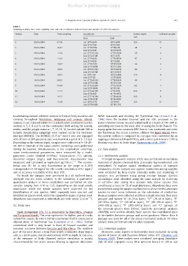
Table 1
Sampling stations, date, time sampling, start and end coordinates, bottom depth and number of collected samples.
Station Date Time sampling Coordinates Bottom depth Collected samples
(m)
Start End
1 09/10/2004 07.58 Lat. 38°03.00N 38°01.84N 250 10
Lon.12°22.76E 12°22.39E
2 09/10/2004 10.47 Lat. 37°58.50N 37°58.23N 48 4
Lon.12°22.94E 12°23.003E
3 09/10/2004 11.54 Lat. 37°53.012N 37°52.934N 25 4
Lon.12°22.534E 12°21.87E
4 09/10/2004 13.36 Lat. 37°54.82N 37°55.605N 87 6
Lon.12°14.99E 12°14.98E
5 09/10/2004 15.04 Lat. 37°59.55N 38°00.456N 66 6
Lon.12°15.103E 12°15.139E
6 09/10/2004 16.05 Lat. 38°03.075N 38°03.865N 86 7
Lon.12°14.976E 12°14.941E
7 09/10/2004 18.02 Lat. 38°01.2N 38°03.018N 330 8
Lon.12°07.1E 12°07.086E
8 10/10/2004 08.02 Lat. 37°56.853N 37°58.816N 88 7
Lon.12°07.236E 12°07.152E
9 10/10/2004 09.40 Lat. 37°53.028N 37°53.922N 102 7
Lon.12°07.187E 12°07.19E
10 10/10/2004 11.13 Lat. 37°52.670N 37°55.55N 630 9
Lon.12°00.10E 11°59.983E
11 10/10/2004 14.13 Lat. 37°57.874N 37°59.482N 310 9
Lon.12°00.024E 12°00.068E
12 10/10/2004 15.30 Lat. 38°02.77N 38°04.4N 355 10
Lon.12°00.042E 12°00.175E

located along inshore–offshore sections in front of Sicily coastline and MAW eastwards and entering the Tyrrhenian Sea (Astraldi et al.,
crossing throughout Marettimo, Favignana and Levanzo Islands. 1996) from the Sardinia Channel, and the LIW, produced in the
Stations 2 and 3 placed within 50 m isobath were considered coastal; Eastern Mediterranean Sea and settled itself at a depth of 100–200 m,
stations 4, 5, 6, 8 and 9, on the continental shelf among the islands, spreading out towards the west, after crossing the Sicily Channel. The
neritic; and the pelagic stations 1, 7, 10, 11, 12, located outside 200 m topographic features constrain LIW flow to turn eastwards and enter
isobath. Zooplankton samplings were carried out by the electronic the Tyrrhenian Sea across a section offshore the Egadi Islands. Here,
2
multinet BIONESS. The BIONESS (0.25 m mouth area and equipped the eastern outflow is composed by a unique vein constituted by an
with 10 nets of 200 µm mesh size) was towed at a speed of 1–1.5 m/s. upper part, between 300 and 650 m, and a lower part down to 1100 m
Depending on the bottom depth, samples were collected at 5–10–20– flowing very close to Sicily slope (Sparnocchia et al., 1999).
50–100 m intervals of the water column. Samplings were performed
during the daytime. Simultaneously to the zooplankton samplings, 2.2. Data analysis
some environmental parameters were measured by a multi-
parameter probe (Seabird 911Plus): temperatures (°C), salinity, 2.2.1. Multivariate analysis
dissolved oxygen (mg/L) and fluorescence. Fluorescence was Principal component analysis (PCA) was performed on Euclidean
measured and calculated as equivalent μgChl-a L − 1 . The conven- distances of physico-chemical data, previously log-transformed and
tional unit (F) for in vivo fluorescence in the range of 0–10V normalized. To explore spatial distribution pattern of copepod
3
corresponds to 0–50 mg/m for Chl-a with a resolution of 0.1 mg/m 3 community, cluster analysis was applied. Similarities among samples
and an accuracy variability of less than 10%. were estimated by Bray–Curtis similarity index and clustering of
On board, the samples were preserved in a 4% buffered form- samples was performed using group average linkage. Species
aldehyde and sea water solution. In the laboratory, a qualitative- assemblages were identified using the same analysis by clustering
quantitative analysis of meso-zooplankton was performed on sub- of variables and taking into account only those species that
samples ranging from 1/10 to 1/25, depending on the total sample contributed at least for 5% of total abundance. Abundance data were
abundance, while the whole samples were observed for the transformed using the square root function to allow the less abundant
identification of rare species. Adult copepods were counted and species to exert some influence on the calculation of similarities.
identified at species level, while the copepodite stages at genus level. Because samples were collected at different depth intervals, they were
Abundance was expressed as individuals per cubic meter (ind.m −3 ). grouped and named “A” (0–20 m layer), “A*” (20–40 m layer), “B”
(40–60 m layer), “C” (60–80 m layer), “D” (80–100 m layer), “E”
2.1. Study area (100–200 m layer), “F” (200–300 m layer) and “G” (groups all
the intervals greater than 300 m). Similarity percentage analyses
Egadi Archipelago (Fig. 1) is constituted by Marettimo, Levanzo (SIMPER) were used to identify those species that contributed most
and Favignana Islands. This area represents the highest part of a wide to similarities between groups and across positions. Primer Beta 6
submarine canyon, by which Sicilian continental shelf is connected to package was used for all of the above-mentioned analysis. All these
abyssal plane of Tyrrhenian Sea (Colantoni et al., 1993). Sicilian analysis were performed only on adult copepods.
continental shelf is very broad in front of Trapani coastline and
becomes narrower between Levanzo and Marettimo. The northern 2.2.2. Univariate analysis
part of this zone shows a drop from which continental slope begins Moreover, some aspects of biodiversity were evaluated by using
and, in a short space, reaches and exceeds 1000 m depth. In this area, species richness (d) and Shannon–Wiener index (H′)(Shannon and
at the entrance of Sicily Channel, surface circulation is mainly Weaver, 1963). These indices were calculated averaging abundance
characterized by two water masses flowing in opposite directions: data of adult copepods every 20 m intervals from 0 to 100 m and