Page 4 - angeo-21-299-2003

302 R. Sorgente et al.: Seasonal variability in the Central Mediterranean Sea circulation

The seasonal variability of the two flows is significantly dif- et al., 1988; Astraldi et al., 1996). Its core depth varies sea-
ferent. The southern flow along the African coast reaches sonally with the LIW being deeper in winter, below 200 m,
its maximum in late fall (Astraldi et al., 1996). The MAW and closer to the surface in summer and autumn (Astraldi
vein close to the southern Sicilian coast is most conspicu- et al., 1999; Sparnocchia et al., 1999). In the Tyrrhenian Sea
ous during summer and autumn, proceeding eastward along the LIW flows along the Italian coast, partially exiting north-
the swift topographically controlled AIS. During winter, the ward from the Corsica Channel, especially during winter, and
MAW fills the whole extent of the Strait up to the western- partially southwestward along the eastern Sardinian coast at
most tip of the southern Sicilian shelf. Starting from spring, a depth between 700–1000 m, then overlying the WMDW-
this MAW then starts to progressively detach from the sur- Western Mediterranean Deep Water in the Sardinia Channel
face, taking the form of a subsurface core at a depth of about (Hopkins, 1978).
60 m in autumn.
3 Model setup
2.2 The intermediate water
3.1 General
The LIW is formed mainly in the northeastern Levantine
basin during winter as a result of cooling and evaporation The model used in this study is based on the Princeton Ocean
processes (Nittis and Lascaratos, 1998). After formation, Model (POM), a three-dimensional primitive equation, fi-
the LIW spreads westward at an intermediate depth, pene- nite difference hydrodynamic model. The POM is a free
trating over the Central Mediterranean ridge and eventually surface, baroclinic, sigma-coordinate model that uses a time
entering the western basin after crossing the Strait of Sicily. splitting technique to solve depth integrated and fully three-
The LIW enters the Sicily Channel through the Medina sill dimensional equations with different time steps. It solves the
with a salinity of about 38.74–38.75 psu and a temperature equation of continuity (1), motion (2, 3 and 4), conservation
of about 14.0–14.1◦C in autumn-winter (Warn-Varnas et al., of temperature (5), salinity (6) and assumes hydrostaticity
1999). It crosses the Strait of Sicily with its core at about and the Boussinesq approximation. The equation of state (7)
250 m and 270 m at each of the two sills. Then the whole is an adaptation of the UNESCO equation of state revised by
LIW moves into the Tyrrhenian Sea, constrained by the topo- Mellor (1991).
graphic features and the Coriolis effect, and partially mixes
with the upper and lower waters, becoming saltier (Sparnoc- The basic equations of the ocean model are written in or-
chia et al., 1999). The flux of LIW is not constant but subject thogonal cartesian coordinates, with x increasing eastward,
to a seasonal variability and calculated to be 2–3 times higher y increasing northward and z increasing vertically upward,
in winter (3.2 Sv) with respect to summer (1.5 Sv) (Manzella and synthetically described by the following equations:

∂u ∂v ∂w (1)
+ + =0 (2)
(3)
∂x ∂y ∂z (4)
(5)
∂u ∂u ∂u ∂u 1 ∂p ∂ ∂u ∂ ∂u ∂ ∂u ∂v (6)
+ u +v +w −fv = + KM ∂x + 2AM ∂x + AM + (7)
∂t ∂x ∂y ∂z ρ ∂x ∂z ∂x ∂y ∂y ∂x

∂v ∂v ∂v ∂v 1 ∂p ∂ ∂v ∂ ∂v ∂ ∂u ∂v
+ u +v +w +fu = KM ∂z + 2AM ∂y + AM ( ∂y + )
∂t ∂x ∂y ∂z ρ ∂y ∂z ∂y ∂x ∂x

∂p
ρg = −

∂z

∂θ ∂θ ∂θ ∂θ ∂ ∂θ ∂ ∂θ ∂ ∂θ
+ u +v +w = KH ∂z + AH ∂x + AH ∂y
∂t ∂x ∂y ∂z ∂z ∂x ∂y

∂S ∂S ∂S ∂S ∂ ∂S ∂ ∂S ∂ ∂S
+ u +v +w = KH ∂z + AH ∂x + AH ∂y
∂t ∂x ∂y ∂z ∂z ∂x ∂y

ρ = ρ (T , S, p)

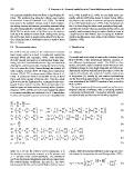
where (u, v, w) are the velocity vector components, ρ is scheme, while the horizontal diffusion terms (AM ) are calcu-
the density, g is the gravity constant, p is the pressure and lated using the Smagorinsky formula (Smagorinsky, 1993),
f = 2 sin ϕ is the Coriolis parameter. The variables θ
and S are the potential temperature and salinity, respectively. ∂v ∂u 2
The vertical mixing coefficients, KM and KH , are calcu- ∂x ∂y
lated using the Mellor and Yamada (1982) turbulence closure ∂u 2 + ∂v 2
+ ,
AM = C x y 2 + (8)
∂x ∂y