Page 6 - angeo-21-299-2003

304 R. Sorgente et al.: Seasonal variability in the Central Mediterranean Sea circulation

(a)A) model. The open boundary data are applied to the high reso-
lution model by linearly interpolating 10-day averaged con-
39 secutive fields.

38 3.5 Surface and bottom boundary conditions

37North Latitude At the free surface, the climatological atmospheric forcing
fields are the same as those used for the coarse model. This
36 atmospheric forcing data set consists of heat and water flux
fields, and wind stress components, on a monthly basis, de-
35 rived from the European Center for Medium Weather range
Forecast 6-hourly Re-Analysis (ERA) data set covering the
34 period 1979–1993 for the whole Mediterranean Sea (Korres
and Lascaratos, 2003). These fields are interpolated into the
33 model grid using a bi-linear interpolation scheme.

32 0.1 N/m2 The surface boundary conditions include the momentum,
9 10 11 12 13 14 15 16 17 heat and net volume fluxes. The momentum surface bound-
East Longitude ary condition adopted is:

(b)B) ∂u τ (15)
KM ∂z |z=η = ρ0
39
where τ is the wind stress monthly mean climatology and ρ0
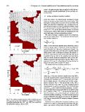
38 is the air density. Figure 3 shows the wind stress fields ob-
tained from the ERA data set in February and August. The
37 structure of the wind stress over the basin is mainly westerly
during winter, with a weakening in summer. The annual cy-
36 cle of the mean east-west and north-south ERA wind stress
amplitudes (Fig. 4), used for the perpetual year simulation,
35 does not contain stochastic components such as from vari-
abilities associated with low pressure systems. This is a con-
34 sequence of the use of a climatological forcing obtained by
using a time series with a length of 14 years.
33
The adopted heat flux boundary condition is:
32 0.1 N/m2
9 10 11 12 13 14 15 16 17 ∂T Qsol − Qup + C1 Tz=0 − Tz=η (16)
East Longitude KH ∂z |z=η = ρ0Cp ρ0Cp (17)
North Latitude
Fig. 3. The monthly averaged wind stress fields in (a) February and ,C1 = ∂Q = 5W m−2 0 C −1
(b) August derived from the ECMWF Re-Analysis (ERA) data set ∂T
covering the period from Jan. 1979 – Dec. 1993. One vector every
four grid points is plotted. Units are N/m2. where Qsol is the solar radiation monthly mean from ERA,
Qup is the upward heat flux computed from the coarse model
perpetual year simulation and Cp is the specific heat capac-
ity at constant pressure. The annual cycle of these compo-

nents is shown in Fig. 5. The second term in Eq. (16) is

the flux correction term, where Tz=0 is the monthly averaged
climatological sea surface temperature from the Med6 data

set and Tz=η is the model first level temperature. Sensitiv-
ity studies performed on the model indicate an optimal value
for C1 equal to 5 W m−2 0C−1. In this way the heat flux is
forced to produce a sea surface temperature consistent with

the Med6 monthly climatology. The Med6 monthly mean sea

surface temperature and salinity are based on the MEDAT-

LAS data set using the MODB analysis technique (Brasseur

et al., 1996).

Similarly for the salinity flux boundary condition, a cor-

rection term is used to ensure that the fresh water flux pro-

duces a sea surface salinity field consistent with the ERA