Page 7 - Antonellini_2013

M. Antonellini et al. / Marine and Petroleum Geology xxx (2013) 1e16 7

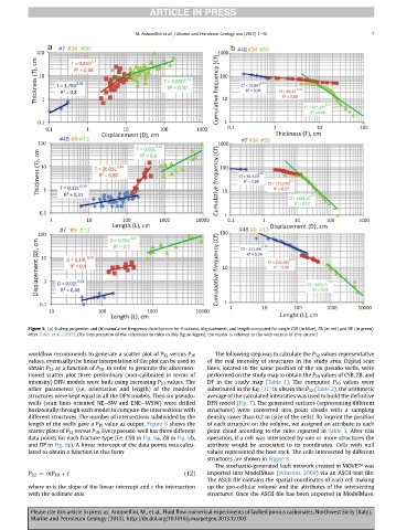
Figure 5. (a) Scaling properties and (b) cumulative frequency distributions for thickness, displacement, and length computed for single CSB (in blue), ZB (in red) and DF (in green).
After Tondi et al. (2012). (For interpretation of the references to color in this figure legend, the reader is referred to the web version of this article.)

workflow recommends to generate a scatter plot of P 32 versus P 10 The following step was to calculate the P 32 values representative
values, eventually the linear interpolation of the plot can be used to of the real intensity of structures in the study area. Digital scan
obtain P 32 as a function of P 10 . In order to generate the aforemen- lines, located in the same position of the six pseudo-wells, were
tioned scatter plot three preliminary (non-calibrated in terms of performed on the study map to obtain the P 10 values of CSB, ZB, and
intensity) DFN models were built using increasing P 32 values. The DF in the study map (Table 1). The computed P 10 values were
other parameters (i.e. orientation and length) of the modeled substituted in the Eq. (11) to obtain the P 32 (Table 2), the arithmetic
structures were kept equal in all the DFN models. Then six pseudo- average of the calculated intensities was used to build the definitive
wells (scan lines oriented NEeSW and ENEeWSW) were drilled DFN model (Fig. 7). The generated surfaces (representing different
horizontally through each model to compute the intersections with structures) were converted into point clouds with a sampling
different structures. The number of intersections subdivided by the density lower than 0.2 m (size of the cells). To imprint the position
length of the wells gave a P 10 value as output. Figure 6 shows the of each structure on the volume, we assigned an attribute to each
scatter plots of P 32 versus P 10 . Every pseudo-well has three different point cloud according to the rules reported in Table 3. After this
data points for each fracture type (i.e. CSB in Fig. 6a, ZB in Fig. 6b, operation, if a cell was intersected by one or more structures the
and DF in Fig. 6c). A linear intercept of the data points was calcu- attribute would be associated to its coordinates. Cells with null
lated to obtain a function in this form: values represented the host rock. The cells intersected by different
structures are shown in Figure 8.
The stochastic-generated fault network created in MOVEÔ was
P 32 ¼ mP 10 þ c (12) imported into ModelMuse (Winston, 2009) via an ASCII text file.
The ASCII file contains the spatial coordinates of each cell making
where m is the slope of the linear intercept and c the intersection up the geo-cellular volume and the attributes of the intersecting
with the ordinate axis. structures. Once the ASCII file has been imported in ModelMuse,

Please cite this article in press as: Antonellini, M., et al., Fluid flow numerical experiments of faulted porous carbonates, Northwest Sicily (Italy),
Marine and Petroleum Geology (2013), http://dx.doi.org/10.1016/j.marpetgeo.2013.12.003