Page 5 - Habitat_Selection_2014

Habitat Selection Response of Anchovy and Sardine

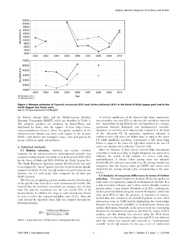
Figure 2. Biomass estimates of Engraulis encrasicolus (E.E.) and Sardina pilchardus (S.P.) in the Strait of Sicily (upper part) and in the
North Aegean Sea (lower part).
doi:10.1371/journal.pone.0101498.g002

the Kinetic Energy (KE), and the Mediterranean Absolute To test the significance of the observed QI values, randomiza-
Dynamic Topography (MADT), which are described in Table 2. tion procedure was used [33] to calculate the confidence intervals
The altimeter products are produced by Ssalto/Duacs and (CI – dashed lines in QI plots) for the null hypothesis (i.e. random
distributed by Aviso, with the support of Cnes (http://www. association between biological and environmental variable).
aviso.oceanobs.com/duacs/). Since the spatial resolution of the Avoidance or selection were subsequently evaluated on the basis
aforementioned dataset was lower with respect to the acoustic of the calculated CI. In particular, significant selection is
EDSU, each dataset was resampled using 1 nmi grid spacing by evidenced when QI values are higher than or equal to the upper
means of bilinear spline interpolation. CI, while significant avoidance corresponds to QI values lying
below or equal to the lower CI. QI values between the two CI
3. Statistical methods curves are interpreted as tolerance behavior [33].
3.1 Habitat selection. Anchovy and sardine selection Since the biomass of both species showed high inter-annual
behavior for the abovementioned environmental variables was variability in both areas (Fig. 2), higher biomasses are expected to
evaluated considering the two study areas in the period 2002–2010 influence the results of QI analysis. To reduce such bias,
for the Strait of Sicily and 2003–2008 for the North Aegean Sea. standardization of density values among years was adopted.
The Single Parameter Quotient analysis [8,9,22,33,34] was used Specifically, for each year and study area, the average density was
computed; then the density values per EDSU and survey were
to investigate the ‘‘mean’’ spatial behavior of species in the specific
temporal windows. To this aim, QI analysis was performed on two divided by the average density value corresponding to the same
survey.
datasets, one for each study area, composed by all data (per
3.2 Analysis of ecosystem differences in terms of habitat
EDSU) pooled.
The first step in applying quotient analysis was the identification selection. Principal Component Analysis (PCA) was applied in
each study area separately, using all environmental variables. It is
of the specific class intervals for each environmental variable. We
a data reduction technique and is often used to identify common
ensured that the minimum occurrence per category was not less
than 5% and the maximum one did not exceed 25% of all pattern within a large dataset. Zwolinski et al. [35], analyzing the
sardine potential habitat along the western Portuguese continental
measurements. In addition the range in each interval was chosen
shelf, used PCA to infer the presence of structures in environ-
in order to reflect the regional variability [sensu 22,34]. Thus, for mental data and considered the identified pattern as main effect
each interval the Quotient index (QI) was obtained through the
(interaction term) in GAM models, highlighting the relationships
following formula:
between the structured variability of environmental dataset and
sardine distribution. Similarly, in the present work the relationship
%Observed Biomass between the environmental patterns, identified by means of PCA
QI i ~
Env:Var:freq i |100 analysis, and fish density was assessed using the PCA factor
coordinates (i.e. the observation values on each PCA axis obtained
where i represents the i-th frequency histogram interval. after the system was rotated and centered) as ‘‘environmental
variable’’ in the QI analysis. In this way a sort of multivariate
PLOS ONE | www.plosone.org 5 July 2014 | Volume 9 | Issue 7 | e101498