Page 7 - Patella_ferruginea_Casu_Rivera_ali2011

Genetica (2011) 139:1293–1308 1299

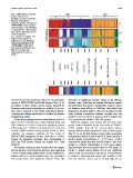
Fig. 3 ISSR dataset: estimated SCR SAS
genetic structure in P.
A A C
ferruginea as inferred using the a B B
Bayesian model-based
clustering analysis. a Results of st
STRUCTURE, and b results of 1
BAPS analyses. Each individual
is represented by a thin vertical
line, which is partitioned into K- nd
coloured segments STRUCTURE 2
(K = number of clusters). The
height of each segment is
proportional to the individual rd
estimated membership in the 3
corresponding cluster. Black
lines separate individuals from
different sampling sites.
Abbreviations are given in
Table 1

ACS,APS,APB CDN,IPO ARG MVE PLF,NAQ MAD,PIT,CGR MLA,MLT GAL,CAR,TIZ,BOF LIT,DIQ,DES,PAR,CRL ALB MEL,CHA,HAB,PLA,CAP ZEM,PAN,MAR,FAV

b
BAPS

resemble the genetic groupings retrieved in the subsequent decreased to significant negative values in the 200 km
rounds of STRUCTURE and BAPS analyses (Fig. 4b–d). distance class. Following an upward fluctuation, spatial
According to these results, genetic groups retrieved by autocorrelation decreased to significantly negative values
Bayesian-model based clustering are unlikely to be arte- for distances from 600 up to 1,000 km, after which they
facts due to violation of the model assumptions (Hardy– displayed a stochastic pattern. These two troughs involved
Weinberg and linkage equilibrium) or isolation by distance many pairwise comparisons between samples from the
(Guillot et al. 2009). clusters A and B in the SCR group as well as between the
All the three grouping schemes tested with the AMOVA SCR group and the cluster C (the SAS group).
(SAS and SCR; Alboran Sea, Siculo-Tunisian Strait, and When the samples were divided into the three main
SCR; clusters A, B and C) showed a significant genetic genetic clusters identified by the first round of STRUC-
differentiation (P \ 0.001) at the highest level of genetic TURE analyses (Fig. 3a), the autocorrelation indices
structure (differentiation among groups) (Table 4). Nev- showed different spatial patterns for each of these groups
ertheless, the grouping matching the first round of (Fig. 5b–d). In the first distance class (within population
STRUCTURE maximised the U CT value (U CT = 0.301). comparisons) clusters A and B (the SCR group) showed a
Among the remaining groupings, that corresponding to positive spatial autocorrelation (r = 0.151 and r = 0.128,
SAS and SCR groups showed the highest U CT value respectively) greater than that found in cluster C (the SAS
(Table 4). group) (r = 0.047). Nevertheless in SCR group spatial
The Mantel correlogram that included all of the samples autocorrelation fell more quickly than in SAS group. In
did not display a clear monotonic decrease, thus suggesting cluster A spatial autocorrelation fell to non significant
a more complex spatial pattern than a simple isolation-by- values in the second distance class (up to 15 km) whereas
distance (IBD) or a clinal variation (Fig. 5a). The pattern in cluster B autocorrelation values were positive in the
was partly clinal, with significant positive values that first two distance classes (up to 15 km) (Fig. 5b, c).

123