Page 11 - Sea-level change_2004

ARTICLE IN PRESS
K. Lambeck, A. Purcell / Quaternary Science Reviews 24 (2005) 1969–1988 1979

results such as these provide a guide to which observa-
tion sites andwhich epochs are most important for
ensuring separability of mantle parameters.

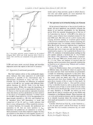
5. The equivalent sea-level function during Late Holocene
Of the potential limitations of the sea-level prediction
model, the most significant one probably concerns the
choice of esl function, particularly for the Holocene
period. With the assumed disappearance of the last of
the Laurentian ice sheet at 6.8 ka BP in the above ice
models, ocean volumes have remained constant for the
past 6800 years. But there are no a priori reasons why
ongoing Antarctic melting or mountain glacier decay
couldnot have resultedin ocean volumes increasing into
Late Holocene time. For example, recent evidence from
Mary Byrd Land, Antarctica, indicates that a significant
lowering of the ice surface has occurredin Late
Holocene time over a large area andthat this may have
contributedas much as 1 m to global level (Stone et al.,
2003). Or, estimates of mountain glacier melting for the
Fig. 5. Ice-volume equivalent sea-level function for the northern
European (NE-1, NE-2) andNorth American (NA-1, NA-2) ice past century indicate a sea-level rise of 0.2–0.4 mm/
models. NE-2 and NA-2 are components of the global nominal ice year (Meier, 1993; Oerlemans, 1999) which, if represen-
model. tative of the past 7000 years, wouldresult in an esl rise
of 1.5–3 m. Thus, our analyses of sea-level data for
rheology andice parameters have generally included the
LGM andmore recent sea-level change andshoreline esl function as an unknown (e.g. Nakada and Lambeck,
migration across the region at this level of accuracy. 1987; Lambeck, 2002).
Across the Mediterranean, there are localities where,
4.5. Separation of earth-model parameters at different times, the predicted values are equal to the
esl values anddata from these localities are particularly
The brief analysis above of the earth-model depen- valuable for estimating corrections to this latter func-
dence indicates that some separation of earth-model tion. For example, at 6 ka BP, the predicted levels along
parameters is possible if the observational data is the Levant coast are nearly zero (Fig. 2f) andany
appropriately distributed in space and time. As an observedlevels from these localities shouldprovide a
example, Fig. 8a illustrates the difference in predicted quite direct measure of the esl value for that epoch. At
values at 6 ka BP for two models with different litho- 12 ka BP, the model esl value is 54 m andthis contour
spheric thickness H 1 (E4–E5, Table 1) for the Medi- in Fig. 2e identifies locations, such as along the northern
terranean region. Within this range the dependence of Tyrrhenian coast of Italy or in the Golfe du Lion, where
the predicted levels on H 1 is approximately linear (Fig. any observations should provide a direct measure of the
10, below) so that the zero contour represents locations esl value. Similarly, at 20 ka BP, the relative sea level
where the relative sea-level predictions are least sensitive equals the esl value at locations such as near Malta and
to the choice of lithospheric thickness. A similar result Lampedusa or the Balearic Islands. These locations will
for 6 ka BP is illustratedin Fig. 8b for the dependence on vary with earth-model parameters and the challenge will
upper-mantle viscosity Z (E1–E3), andlocations can be to identify locations where the isostatic terms are
um
be identified where this dependence is small and both small andinsensitive to at least some of the mantle
comparison of the H 1 and Z results indicates that parameters.
um
there is some orthogonality of these sensitivity contours. Consider observed sea level Dz o at two locations j ,
1
In western Sardinia, for example, the predictions are j for the same epoch t andfar from former ice sheets
2
insensitive to H 1 but are more sensitive to Z um . such that the total isostatic corrections Dz I are small.
Elsewhere, the predictions are insensitive to either of Then
these parameters within their respective ranges, but they
Dz o ðj ; tÞ¼ Dz esl ðtÞþ Dz I ðj ; tÞ,
are sensitive to the choice of lower mantle viscosity (c.f. 1 1
Fig. 8c), such as along the coast of North Africa, and Dz o ðj ; tÞ¼ Dz esl ðtÞþ Dz I ðj ; tÞ,
2
2