Page 9 - Sea-level change_2004
P. 9
ARTICLE IN PRESS
                                  K. Lambeck, A. Purcell / Quaternary Science Reviews 24 (2005) 1969–1988  1977

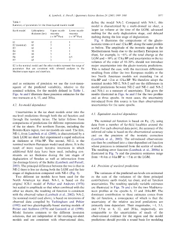
          Table 1                                             define the model NA-2. Compared with NA-1, this
          Summary of parameters for the three-layeredmantle model
                                                              model is characterized by a multi-domed ice sheet, a
                                                              larger ice volume at the time of the LGM, advanced
          Earth model  Lithospheric  Upper mantle  Lower mantle
                      thickness (km)  viscosity  viscosity    melting for the early deglaciation stage, and delayed
                                       20
                                                   22
                                   (   10 Pa s)  (   10 Pa s)  melting during the late stage of deglaciation.
                                                                Fig. 6 illustrates the comparisons of the glacio-
          El          65           2           1
          E2 (nominal)  65         3           1              isostatic terms at 6 and12 ka BP, along the same profiles
          E3          65           4           1              as before. The amplitude of the isostatic signal in the
          E4          50           3           1              Mediterranean basin due to the northern European ice
          E5          80           3           1              sheet, for example, is  6% of the total change at the
          E6          65           3           0.5            LGM and  10% at 12 ka BP anduncertainties in the ice
          E7          65           3           2
                                                              volumes of the order of 10–20% should not introduce
          E2 is the nominal model and the other models represent the range of  major uncertainties into the glacio-isostatic predictions.
          parameters that are consistent with reboundanalyses in the  This is indeed the case, with the maximum differences
          Mediterranean region and elsewhere.
                                                              resulting from either the two European models or the
                                                              two North American models not exceeding 1 m at
                                                              6 ka BP and  2 m at 12 ka BP. We therefore adopt the
          andas estimates of precision we use the root-mean-  nominal models NE-2, NA-2 and use the differences in
          square of the predicted variability, relative to the  model predictions between NE-2 and NE-1 and NA-2
          nominal solution, for the models defined in Table 1.  andNA-1 as a measure of uncertainty. This gives the
          Figs. 4e andf illustrate these precision estimates for the  results illustratedin Figs. 6e andf for the two profiles
          two transects at 6, 12, and20 ka.                   andat three epochs. In most cases, the uncertainty
                                                              introduced from this source is less than observational
          4.2. Ice-model dependence                           uncertainties for the same epochs.

           Uncertainties in the ice sheet models enter into the
                                                              4.3. Equivalent sea-level dependence
          sea-level predictions through both the esl function and
          through the isostatic terms. The latter follows from
                                                                The nominal esl function is basedon Eq. (5), using
          comparisons of predictions for different representations
                                                              data from a number of far-field localities around the
          of the ice sheets. For northern Europe, including the
                                                              world. For each observed data point, the accuracy of the
          Barents-Kara region, two ice models are used. The first,
                                                              inferredesl value is based on the observational accuracy
          NE-1, from Lambeck et al. (2000), is characterizedby a
                                                              andon the precision of the isostatic correction
          thick LGM ice sheet that experienceda rapidreduction
                                                              (Lambeck et al., 2002). The esl-reduced observations
          in thickness at 19 ka BP. The second, NE-2, is the
                                                              can then be combined into a time-dependent esl function
          nominal northern European model used above. It is the
                                                              whose precision is estimatedfrom the scatter of results.
          result of more recent iterative inversions in which
          additional field data have been used, including con-  The resulting error function (Lambeck et al., 2004a)is
                                                              illustratedin Fig. 7a andthe precision estimates range
          straints on ice thickness during the late stages of  from  0.4 m at 6 ka BP to  5 m at the LGM.
          deglaciation of Sweden as well as information from
          the drainage history of the Baltic (Lambeck andPurcell,
          2003). The principal difference between the two is that in  4.4. Precision of sea-level predictions
          NE-2 there is less ice during both the LGM and the late
          stages of deglaciation compared with NE-1 (Fig. 5).   The variances of the predicted sea levels are estimated
           Two different ice models have been used for the    as the sum of the variances of the three principal
          North American ice sheet. NA-1, is basedon the      contributions: earth model, ice sheet, and esl function
          original ICE-1 model of Peltier andAndrews (1976)   uncertainties. The resulting spatially variable estimates
          but scaledin amplitude so that when combined with the  are illustratedin Figs. 7b andc for the two Mediterra-
          other ice sheets, the resulting esl function is consistent  nean profiles at the epochs 6, 12 and20 ka BP. The
          with the observedvalues (Lambeck et al., 2002). NA-2,  dominant contribution to these estimates comes from
          the nominal model used above, is based on inversions of  the esl function, a consequence of which is that the
          observeddata compiled by Tushingham andPeltier      uncertainty of the relative sea-level predictions are
          (1992) andtwo glaciologically-based starting models of  primarily time dependent. Their magnitudes,  1, 3.5,
          Peltier andAndrews (1976) and Licciardi et al. (1998).  and5.5 m at 6, 12, and 20 ka, respectively, are
          Model features common to the different inversion    comparable to the uncertainties of much of the
          solutions, that are independent of the starting ice-sheet  observational evidence for the region and the model
          models and are consistent with observational data,  predictions should provide a sound basis for modeling

