Page 6 - Vannucchi_Cappietti_2016

Sustainability 2016, 8, 1300 6 of 21

These areas were selected taking into consideration technical aspects, such as the offshore
Sustainability 2016, 8, 1300
6 of 21
resource availability, and non-technical aspects which, amongst others, are related to the interest of
our research group for sitting a pilot plant.
The model meshes were characterized by a triangular grid size of about 1000 m in water depths
The model meshes were characterized by a triangular grid size of about 1000 m in water depths
over 50 m, 500 m in water depths between 50 m and 30 m, 300 m in water depths between 30 m and
over 50 m, 500 m in water depths between 50 m and 30 m, 300 m in water depths between 30 m and
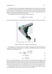
20 m and 200 m from water depth of 20 m until the coast. Figure 2 shows, as an example, the mesh
20 m and 200 m from water depth of 20 m until the coast. Figure 2 shows, as an example, the mesh
used for the Sicily area with resolution information (the total number of computational nodes was
used for the Sicily area with resolution information (the total number of computational nodes was
13,256 and the total number of the elements was 25,506).
13,256 and the total number of the elements was 25,506).
The nearshore wave power (Pw) was computed as in Equation (2)
The nearshore wave power (P w ) was computed as in Equation (2)
2
2π w ∞ w  c
P  g  f,   E , f dfd , (2)
w g
P w = ρg 00 c g(f, θ) × E(f, θ)dfdθ, (2)
0 0
where E is the energy density, cg is the group celerity, f is the wave frequency and θ is the wave
direction.
where E is the energy density, c g is the group celerity, f is the wave frequency and θ is the wave direction.

Figure 2. Sicily model mesh with grid resolution information.
Figure 2. Sicily model mesh with grid resolution information.

The temporal wave power fluctuation was computed, following Cornett [6], as the coefficient of
The temporal wave power fluctuation was computed, following Cornett [6], as the coefficient of
variation (COV) (Equation (3)), the seasonal variability index (SV) (Equation (4)), and the monthly
variation (COV) (Equation (3)), the seasonal variability index (SV) (Equation (4)), and the monthly
variability index (MV) (Equation (5)):
variability index (MV) (Equation (5)):
  2 2  0.5 0.5
  Pt     PP  P − P 
COV  P  COV(P) = σ(P(t))  = , , (3)
(3)

Pt
 µ(P(t)) P P
P S1 − P S4
SV = , (4)
P P P S4
S1
SV  , (4)
P M1 P − P M4
MV = , (5)
P
P  P
where σ is the standard deviation, µ is the mean M1 and the over-bar means the time-averaging. In this
M 4
(5)
MV 
,
P mean wave power for the most energetic season
work, COV is applied to the 3-h time series. P S1 is the
(usually the winter, from December to February), P S4 is the mean wave power for the least energetic
where σ is the standard deviation, μ is the mean and the over-bar means the time-averaging. In this
season (usually the summer, from June to August), the yearly mean power. P M1 is the mean wave
work, COV is applied to the 3-h time series. PS1 is the mean wave power for the most energetic
power for the most energetic month and P M4 is the mean wave power for the least energetic month.
season (usually the winter, from December to February), PS4 is the mean wave power for the least
Relatively lower values of COV, SV, and MV mean a less varying wave power time series,
which helps locate the most promising areas for wave energy harvesting.